Univariate Analysis

Univariate Analysis¶

Welcome to the third video on data exploration. In this one, we will concentrate on the univariate analysis of the given data of the Pronto bike-sharing service.

For this, we start by investigating the different variables individually.

We know already that the dataset contains information on more than 140,000 single trips. By checking the first and last date of the trip data, we see that the information is given for exactly one year.

Additionally, we can check how many single bikes and stations are given in the dataset. With more than 480 bikes at over 50 stations, we expect diverse riding behaviour with interesting inter-dependencies.

As a first analysis, we concentrate on the single trip durations because the trip duration directly affects bike availability and the type of service that can be provided by Pronto.

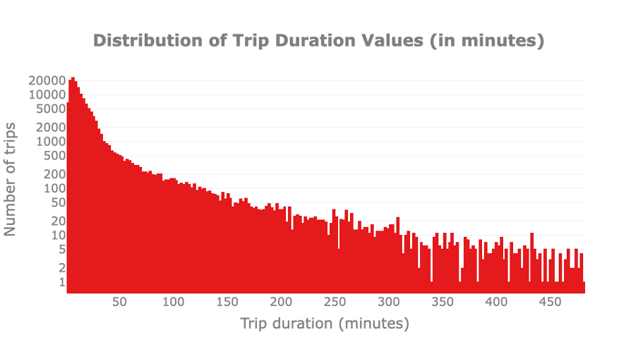
First, we visually check whether there are outliers in trip duration. For this, we plot the distribution of trip durations to spot trips that are much shorter or longer than the remaining ones. Please note that the y-axis is reported in logarithmic scale to improve the readability of the graph.

We observe that bike usage can vary from a few minutes to 480 minutes, or 8h. The latter is probably a limitation due to the service hours of the Pronto service, that is, the maximum amount of time that a bike can be rented during one single day. By just looking at the distribution we cannot notice any anomaly.

In a second step, we have a look at the users’ age as we assume that it influences the bike usage behaviour for example due to health and working status. Consequently, it is relevant to explore the typical users' age. Similarly to the previous analysis, we analyse the age distribution to spot outliers and let potentially interesting insights emerge.

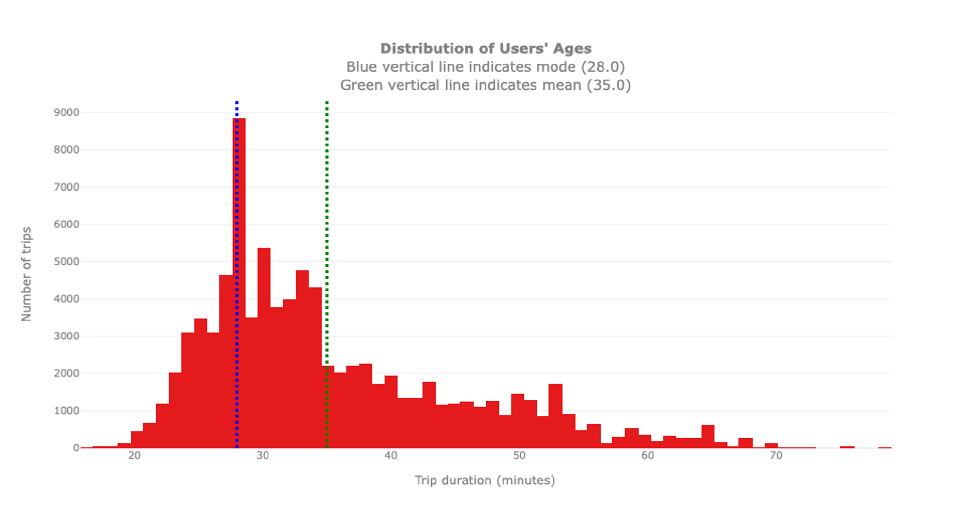
We see that the youngest user is 16 years old, the oldest one 79. As indicated before, please note that these are only the subscribed users. It is possible that younger or older people use the bikes as well but are Short-Term Pass Holders for which no specific information is available. The biggest group of users is 28 years old, hence the mode of the distribution, while the average age is 35. Interestingly, we can notice that the distribution of the ages is not as smooth as expected: An unexpectedly high number of users is 28 years old. To inspect this anomaly, we proceed with an analysis of the birth years.

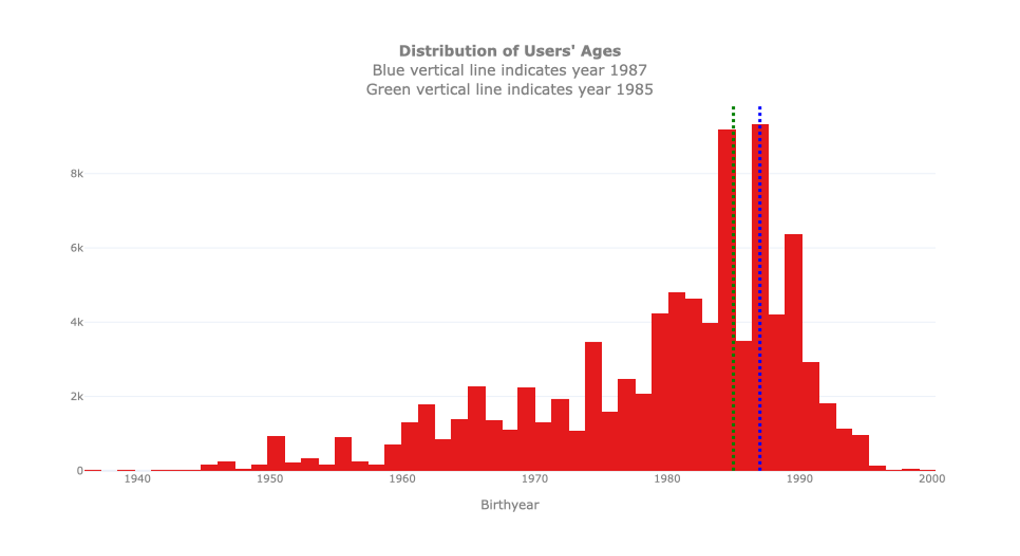
By additionally looking at this distribution, we discover that the anomaly may depend on the users' declared birth year. The histogram indicates that bike rental seems to be quite common for users born in 1985 and 1987, but not for those born in 1986. It is unlikely that these peaks come from a 'baby-boom' in the Seattle area in these specific years. This may depend on a limited number of users born in those years which intensively used the service during the year for example, for a sports club with frequent commuters or a reoccurring city trip organized by some youth association. Unfortunately, the data does not include this type of information. In case you want to dig deeper into this anomaly, you could further analyse whether there are bikes that are frequently moving back and forth from or to the same locations in the same period of time for users that were born in 1985 and 1987. But this is beyond the scope of the univariate exploration.

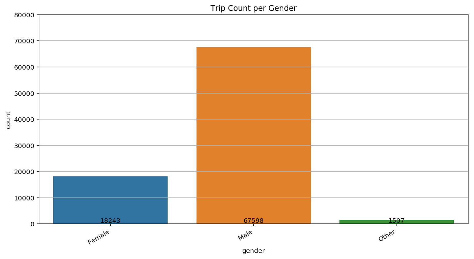
As already discussed in the former video, we also have a look at the gender distribution. Also in this case, we should note that we do not have the identity of the users of each ride. Consequently, we cannot exclude that this bar plot is biased by a limited number of men that used the service with an annual pass while more women use short-term passes. Nevertheless, it is a trend that is observed in many Western cities and is often linked to narrow and sometimes dangerous biking lanes.

Finally, we have a look at the single locations where a bike was rented. The Pronto rental service relies on bike availability at each station. For this reason, it is interesting to explore how bikers used these stations and whether some stations are more popular than others.

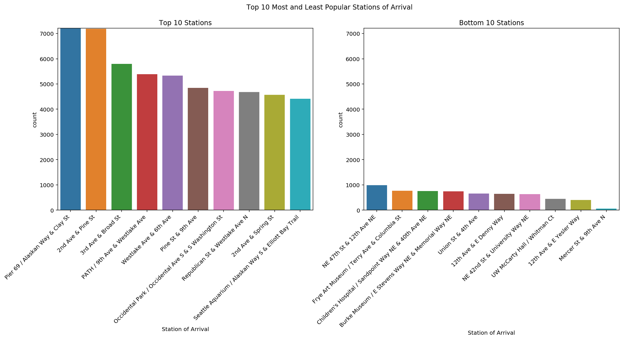
The bar plots shown here provide the top 10 most and least popular stations of arrival. As you can observe, there is a big difference in terms of trips toward these stations. This can lead to unbalanced stations, where extra bikes need to be continuously moved toward stations with missing bikes. This aspect will be further inspected later on in the tutorial.

From this univariate analysis we already learnt several things about the biking - or at least the subscription – behaviour in Seattle. We know already that the average subscriber is male, around 30 and enjoys going to Pear 69.

In the next video, we will expand our analysis to bivariate analysis in order to better understand how two variables influence each other.